Georeferencing Topo Sheets and Scanned Maps (QGIS3)
Most GIS projects require georeferencing some raster data. Georeferencing is the process of assigning real-world coordinates to each pixel of the raster. Many times these coordinates are obtained by doing field surveys - collecting coordinates with a GPS device for few easily identifiable features in the image or map. In some cases, where you are looking to digitize scanned maps, you can obtain the coordinates from the markings on the map image itself. Using these sample coordinates or GCPs ( Ground Control Points ), the image is warped and made to fit within the chosen coordinate system. In this tutorial I will discuss the concepts, strategies and tools within QGIS to achieve a high accuracy georeferencing.
This tutorial is to geo-reference an image which has coordinates information available on the map image itself (i.e. grids with labels). If your source image does not have such information, you can use the method outlined in Georeferencing Aerial Imagery (QGIS3)
Overview of the task
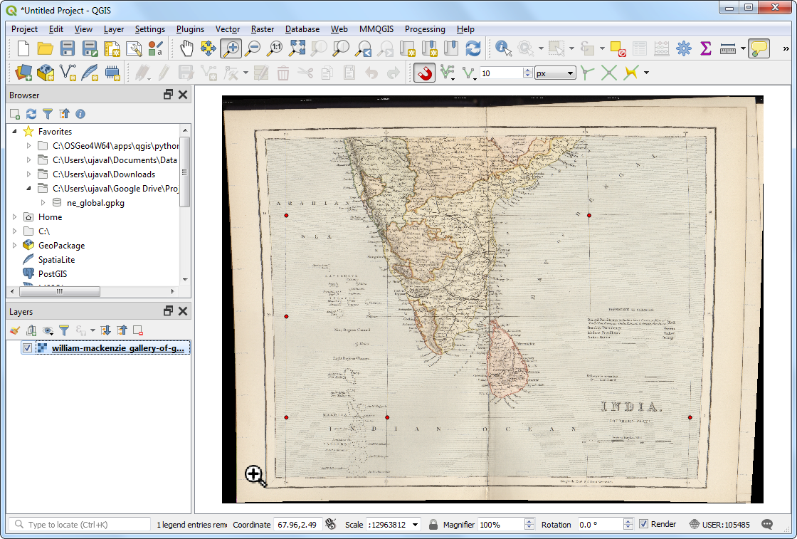
We will use a scanned map of southern India from 1870 and geo-reference it using QGIS.
Other skills you will learn
- How to determine datum and coordinate system for old maps.
Procedure
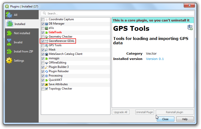
1.Georeferencing in QGIS is done via the Georeferencer GDAL plugin. This is a core plugin - meaning it is already part of your QGIS installation. You just need to enable it. Go to and enable the Georeferencer GDAL plugin in the Installed tab. See Using Plugins for more details on how to work with plugins.
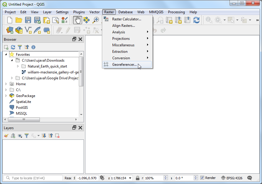
- The plugin is installed in the Raster menu. Click on to open the plugin.
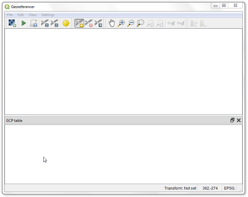
- The plugin window is divided into 2 sections. The top section where the image will be displayed and the bottom section where a table showing your GCPs will appear.
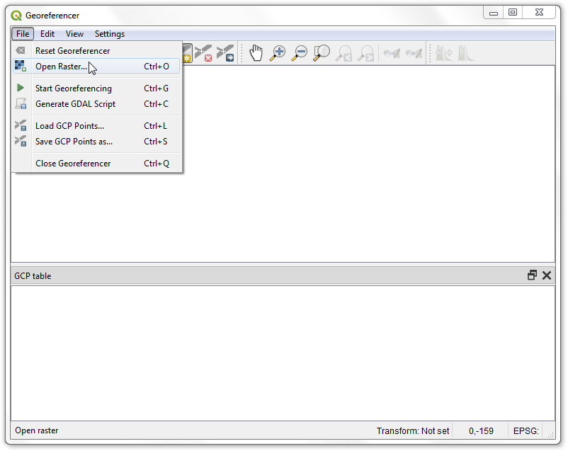
- Now we will open our JPG image. Go to . Browse to the downloaded image of the scanned map and click Open.
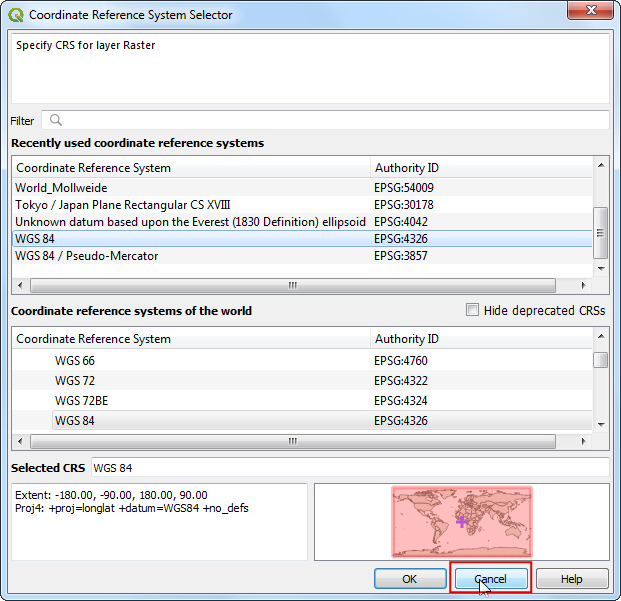
- In the next screen, you will asked to choose the raster’s coordinate reference system (CRS). Our source image is a plain JPEG file and doesn’t have any coordinate reference system atached to it, so you can click Cancel.
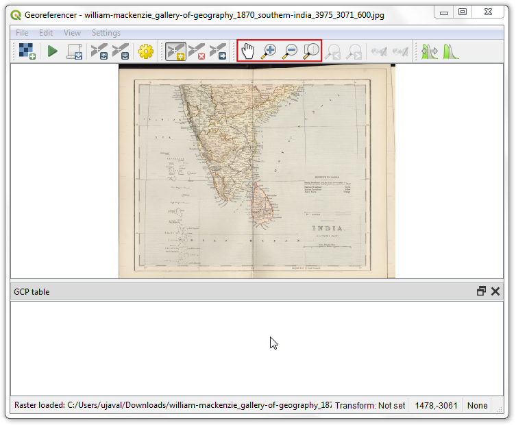
- You will see the image will be loaded on the top section. You can use the zoom/pan controls in the toolbar to learn more about the map.
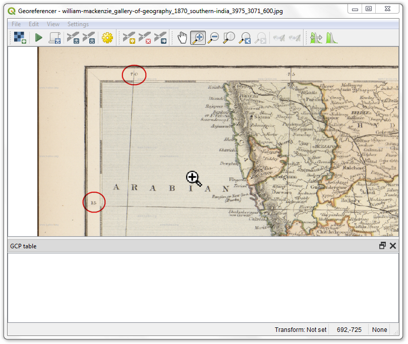
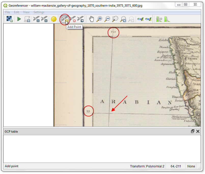
- Now we need to assign coordinates to some points on this map. If you look closely, you will see coordinate grid with markings. These are Latitude and Longitude grid lines.
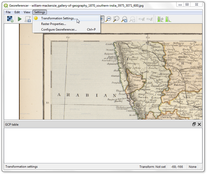
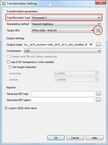
- Before we start adding Ground Control Points (GCP), we need to define the Transformation Settings. Go to .
- In the Transformation settings dialog, choose the Transformation type as
Polynomial 2. See QGIS Documentation to learn about different transofrmation types and their uses. Click Select CRS button next to Target SRS.
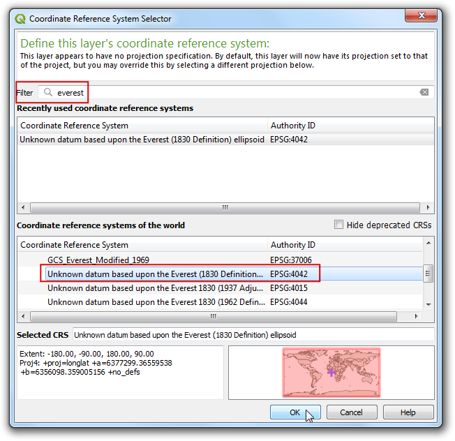
- If you are geo-referencing a scanned map like this, you can obtain the CRS information from the map itself. Looking at our map image, the coordinates are in Latitude/Longitude. There is no datum information given, so we have to assume an appropriate one. Since it is India and the map is quite old, we can bet the Everest 1830 datum would give us good results. Search for
everest and select the CRS with oldest definition of the Everest datum (EPSG:4042). Click OK.
Note
Survey of India Topo Sheets created between the year 1960 and 2000 use the Everest 1956 spheroid and India_nepal datum. If you are georeferencing SOI Topo Sheets, , you can define a Custom CRS in QGIS with the following paramters and use it in this step. This definition includes a delta_x, delta_y and delta_z parameters for transforming this datum to WGS84. See this page for more information on the Indian Grid System.
+proj=longlat +a=6377301.243 +b=6356100.2284 +towgs84=295,736,257,0,0,0,0 +no_defs
Note
Most maps are created using a Projected CRS. If the map you are trying to georeference uses a projected CRS that you know of, but the graticules labels are in a Geographic CRS (latitude/longitude), you may use an alternate workflow to minimize distortion. Instead of using a Geographic CRS like we are using here, you can create a vector grid in QGIS and transform it to the projected CRS to be used as a reference for accurate coordinate capture. See this page for more details.
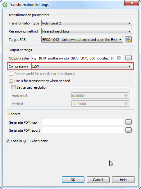
- Name your output raster as
1870_southern_india_modified.tif. Choose LZW as the Compression. Make sure the Load in QGIS when done option is checked. CLick OK.
Note
Uncompressed GeoTIFF files can be very large in size. So compressing them is always a good idea. You can learn more about different TIFF compression options (LZW, PACKBITS or DEFLATE) in this article.
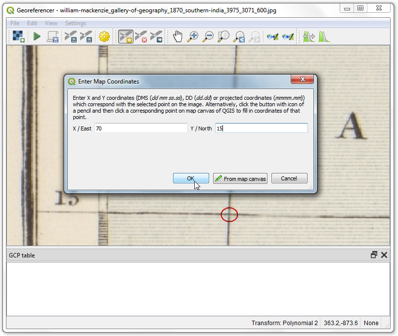
- Now we can start adding the Ground Control Points (GCP). The intersections of the grid lines will serve as the ground-truth in our case. As the grid lines are labeled, we can determine the X and Y coordinates of the points using them. Click Add Point.
13 . In the pop-up window, enter the coordinates. Remember that X=longitude and Y=latitude. Click OK.
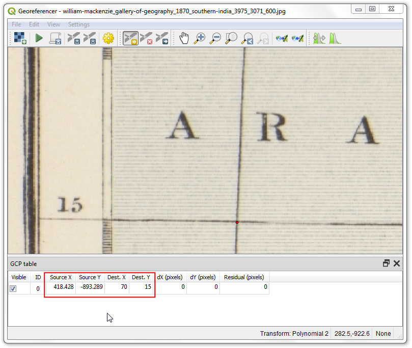
- You will notice the GCP table now has a row with details of your first GCP.
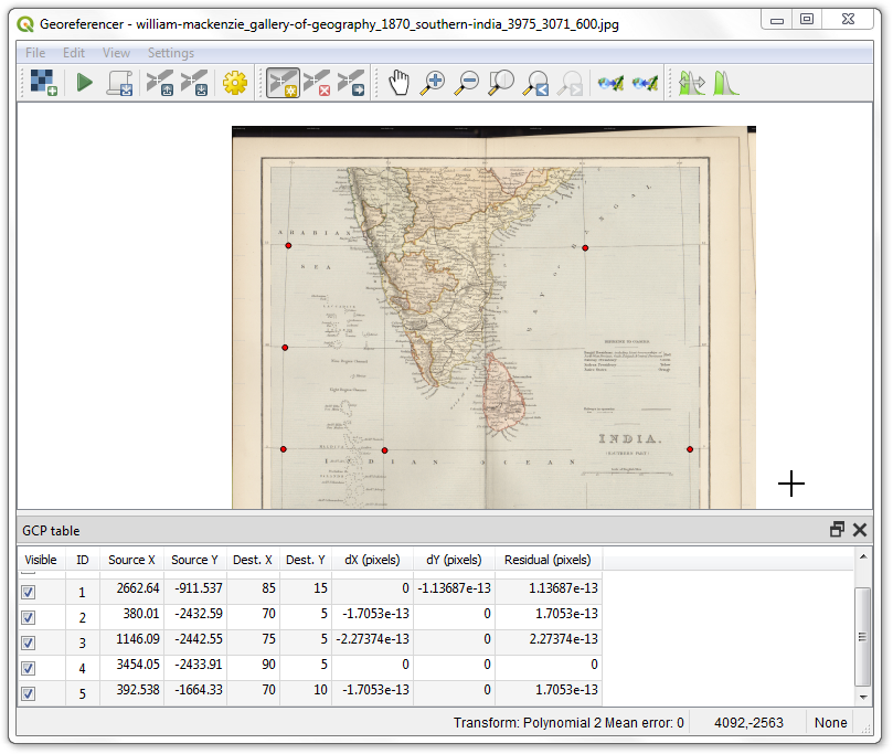
- Similarly, add at least more GCPs covering the entire image. The more points you have, the more accurate your image is registered to the target coordinates. The
Polynomial 2 transform requires at least 6 GCPs.
- Once you have added the minimum number of points required for the transform, you will notice that the GCPs now have a non-zero
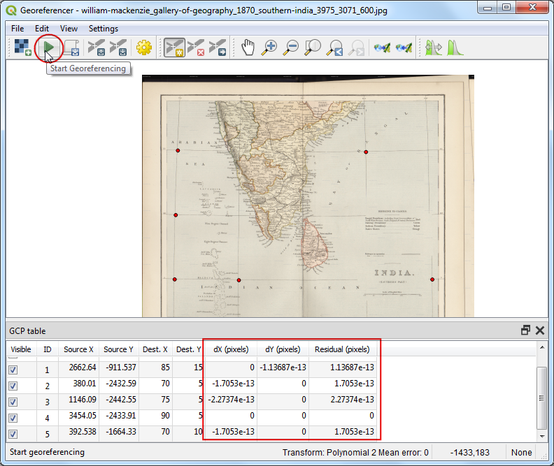
dX, dY and Residual error values. If a particular GCP has unusually high error values, that usually means a human-error in entering the coordinate values. So you can delete that GCP and capture it again. You can also edit the coordinate values in the GCP Table by clicking the cell in either Dest. X or Dest. Y columns. Once you are satisfied with the GCPs, go to . This will start the process of warping the image using the GCPs and creating the target raster.
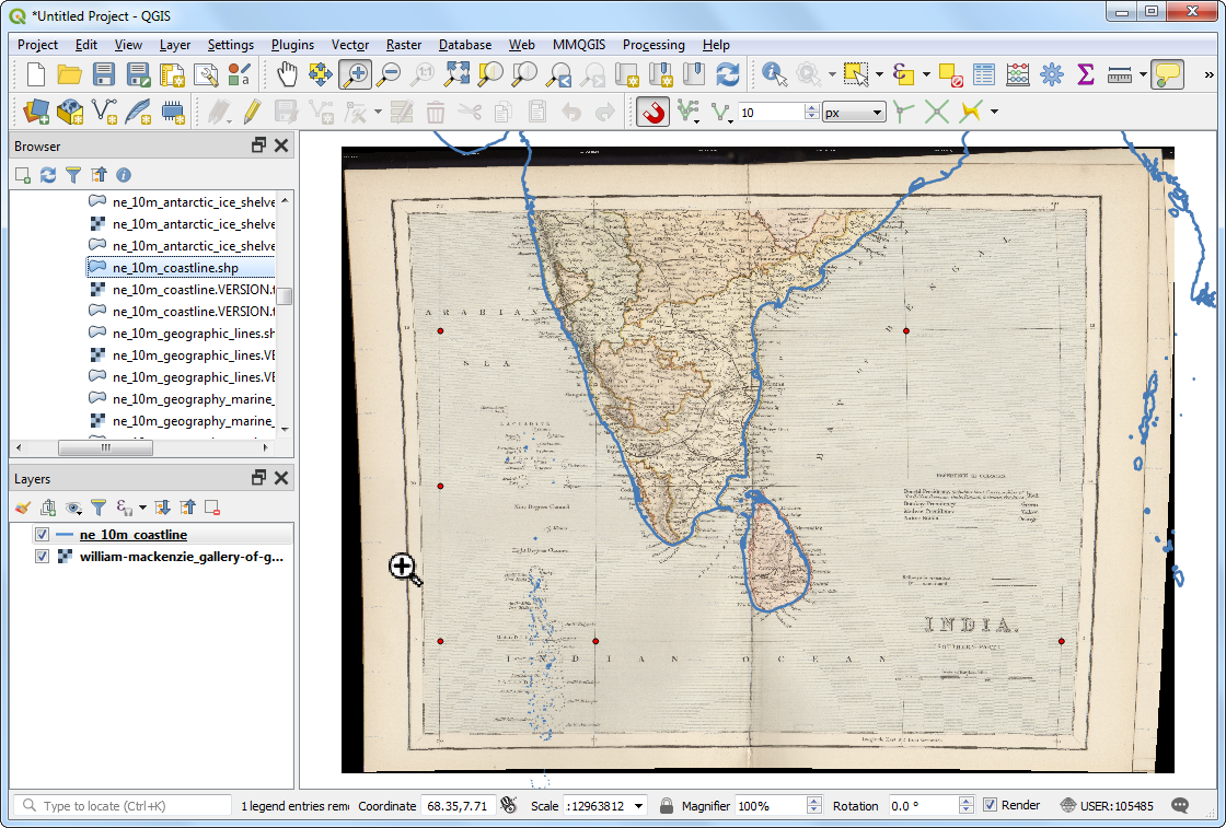
- Once the process finishes, you will see the georeferenced layer loaded in QGIS. The georeferencing is now complete.
Note
The GCPs will also be displayed in the main QGIS Canvas. If you wish to remove them, you can switch to the Georeferencer window, and choose .
- It is a good practice to verify your work. How do we check if our georeferencing is accurate? In this case, you can load the boundary shapefile from a trusted source like the Natural Earth dataset and compare them. You will notice they match up pretty nicely. There is some error and it can be further improved by taking more control points, changing transformation parameters and trying a different datum.