Locating Nearest Facility with Origin-Destination Matrix (QGIS3)¶

In the previous tutorial, Basic Network Visualization and Routing (QGIS3), we learnt how to build a network and calculate the shortest path between 2 points. We can apply that technique for many different types of network-based analysis. One such application is to compute Origin-Destination Matrix or OD Matrix. Given a set of origin points and another set of destination points, we can calculate shortest path between each origin-destination pairs and find out the travel distance/time between them. Such analysis is useful to locate the closest facility to any given point. For example, a logistics company may use this analysis to find the closest warehouse to their customers to optimize delivery routes. Here we use Distance Matrix algorithm from QGIS Network Analysis Toolbox (QNEAT3) plugin to find the nearest health facility to each address in the city.

Note

This tutorial shows how to use your own network data to compute an origin-destination matrix. If you do not have your own network data, you can use ORS Tools Plugin and algorithm ORS Tools ‣ Matrix ‣ Matrix from Layers to do the similar analysis using OpenStreetMap data. See Service Area Analysis using Openrouteservice (QGIS3) to learn how to use ORS Tools plugin.

Overview of the task¶

We will take 2 layers for Washington DC - one with points representing addresses and another with points representing mental health facilities - and find out the facility with the least travel distance from each address.

Other skills you will learn¶

Extract a stratified random sample from a point layer.
Use Virtual Layers to run SQL query on a QGIS layer.
Use Python Console Editor to run a pyqgis script.

Get the data¶

District of Columbia government freely shares hundreds of datasets on the Open Data Catalog.

Download the following data layers as shapefiles.

For convenience, you may directly download a copy of the datasets from the links below:

Street_Centerlines.zip

Address_Points.zip

Adult_Mental_Health_Providers.zip

Data Source: [DCOPENDATA]

Setup¶

Visit Plugins ‣ Manage and Install plugins. Search for QNEAT3 plugin and install it. Click Close.

Procedure¶

Locate the downloaded Street_Centerlines.zip file in the Browser panel. Expand it and drag the Street_Centerlines.shp file to the canvas. Similarly, locate the Adult_Mental_Health_Providers.zip file, expand it and add Adult_Mental_Health_Providers.shp to the canvas.

Next, locate the Address_Points.zip file, expand it and add the Address_Points.shp. You will see a lot of points around the city. Each point represents a valid address. We will not randomly select 1 point in each ward to use as the origin points. This technique is called stratified sampling. Go to Processing ‣ Toolbox.

Search for and locate the Vector Selection ‣ Random extract within subsets algorithm.

Select Address_Points as the Input layer. Each address point contains an attribute called WARD_2012 which has the ward number associated with the address. As we want only 1 point per ward, we use that attribute as the ID field. Set Number/percentage of selected features as 1.

A new layer Extracted (random stratified) will be added to the Layers panel.

Turn-off the visibility for the Address_Points layer. Right-click on the Extracted (random stratified) layer and select Rename layer.

Let’s rename this layer as origin_points. Similarly rename the Adult_Mental_Health_Providers layers representing the health facilities as destination_points. Naming the layers this way makes it easy to identify them in subsequent processing. Go to Processing ‣ Toolbox.

Locate the QNEAT3 ‣ Distance matrices ‣ OD Matrix from Layers as Table (m:n) algorithm. If you do not see this algorithm in the toolbox, make sure you have installed the QNEAT3 plugin.

This algorithm helps find the distances along the network between selected origin and destination layers. Select Street_Centerlines as the Network layer. Select origin_points as the From-Points layer and OBJECTID as the Unique Point ID field. Similarly, set destination_points as the To-Points Layer and OBJECTID as the Unique Point ID field. Set the Optimization Criterion as Shortest Path.

As many streets in the network are one-way, we need to set the Advanced parameters to specify the direction. See Basic Network Visualization and Routing (QGIS3) for more details on how these attributes are structured. Choose DIRECTIONA as the Direction field. Enter One Way (Digitizing direction) as the Value for forward direction and One way (Against digitizing direction) as the Value for backward direction. Keep other options to their default values and click Run.

A new table layer called Output OD Matrix will be added to the Layers panel. Right-click and select Open Attributes Table. You will see that the table contains 117 rows. We had 9 origin points and 13 destination points - so the output contains 9x13 = 117 pairs of origins and destination. The total_cost column contains distance in meters between each origin point to every destination point.

For this tutorial, we are interested in only the destination point with the shortest distance. We can create a SQL query to pick the destination with the least total_cost among all destinations. Go to Database ‣ DB Manager..

In the DB Manager dialog, select the Virtual Layers ‣ Project layers ‣ Output OD Matrix from the left-hand panel. See Virtual layers documentation to learn more. Click the SQL Window button.

Enter the following query and click Execute. The results will be displayed in the panel below. As expected, we have 9 rows in the result - the shortest path destination for each origin point. Check and select Column with unique values as origin_id. Enter nearest_destinations as the Layer name (prefix). Click Load.

select origin_id, destination_id, min(total_cost) as shortest_distance
from 'Output OD Matrix' group by origin_id

A new virtual layer nearest_destinations will be added to the Layers panel. This table has the result of our analysis. Nearest mental health center for each of the 9 origin points. Let’s try a few different ways to visualize and validate these results. Go to Processing ‣ Toolbox. Search for and locate the Join attributes by field value algorithm. Double-click to launch it.

Select origin_points as the Input layer and OBJECTID as the Table field. Set nearest_destinations as the Input layer 2 and origin_id as the Table field 2. Click the ... button next to Layer 2 fields to copy and select destination_id and shortest_distance. Click Run.

A new Joined layer will be added to the Layers panel. This layer has the nearest destination id attribute for each origin point. We can now create a hub-spoke visualization using this layer. Search for Vector analysis ‣ Join by lines (hub lines) algorithm. Right-click to launch it.

Select destination_points as the Hub layer and OBJECTID as the Hub ID field. Select Joined layer` as the :guilabel:`Spoke layer` and ``destination_id as the Spoke ID field. Click Run.

Once the processing finishes, a new layer Hub lines will be added to the Layers panel. This layer shows the lines connecting each origin with the nearest destination.

Note that even though the lines connecting the origin and destination is a straight-line, the destination was found using the distance along the network. It will be much useful visualization to show the actual shortest-path between each origin-destination. As of now, there is no easy way to generate the shortest-path between multiple origin-destination pairs the way we generated the distance matrix. But I will demonstrate a way to use some python scripting to generate this visualization. Firs, let’s run the shortest path algorithm on 1 pair. Locate the QNEAT3 ‣ Routing ‣ Shortest path (point to point) algorithm and launch it.

In the Shortest Path (Point to Point) dialog, select Street_Centerlines as the Vector layer representing network. Keep the Path type to calculate as Shortest. Next we need to pick a start and end point. You can click the ... button next to Start point and click on the origin point in the canvas. Similarly select the destination point as the End point. Expand the Advanced parameter section. Choose DIRECTIONA as the Direction field. Enter One Way (Digitizing direction) as the Value for forward direction and One way (Against digitizing direction) as the Value for backward direction. Keep other options to their default values and click Run.

A new layer Shortest Path Layer wll be added to the Layers panel. You will see that this path follows the network rather than connecting the origin and destination with a straight line. The reason we ran the algorithm on 1 pair is to easily identify the parameter values that we can use in our script. Select both Hub lines and Shortest Path layer, right-click and select Remove Layer. Click the History button in the Processing Toolbox.

Pick the top-most algorithm and you will see the full command displayed in the panel below. Copy the command and click Close.

Go to Plugins ‣ Python Console.

Click the Show Editor button in the Python Console.

In the editor window, copy/paste the following script. This script uses the parameter values from the processing history that we saw earlier. Click Run Script button to start execution.

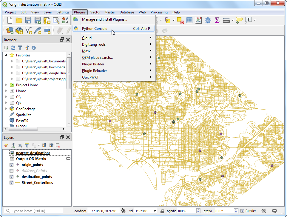
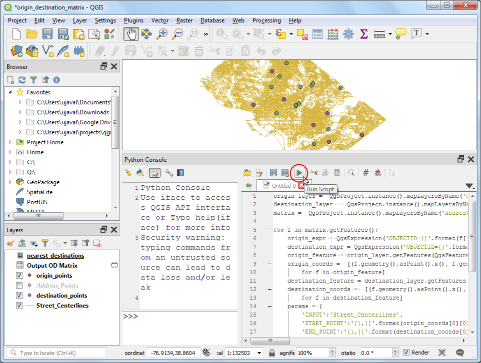
origin_layer =  QgsProject.instance().mapLayersByName('origin_points')[0]
destination_layer =  QgsProject.instance().mapLayersByName('destination_points')[0]
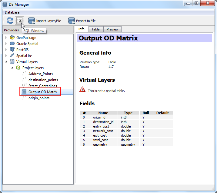
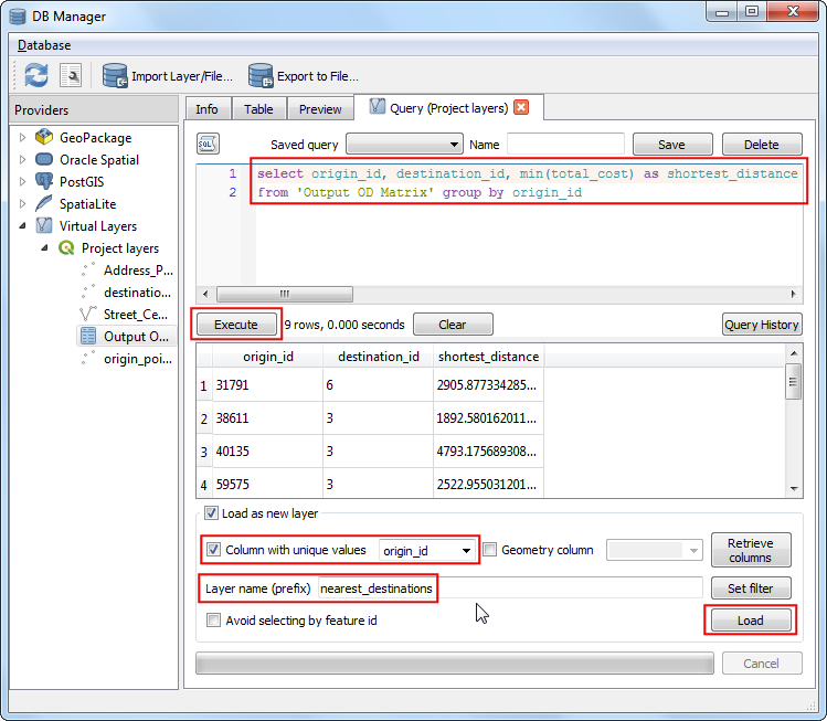
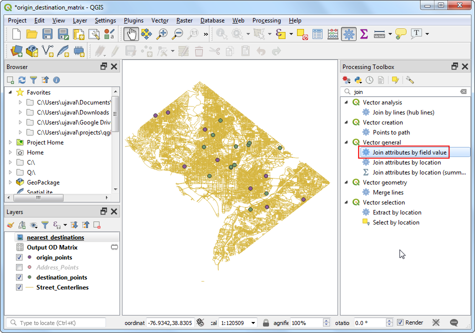
matrix =  QgsProject.instance().mapLayersByName('nearest_destinations')[0]

for f in matrix.getFeatures():
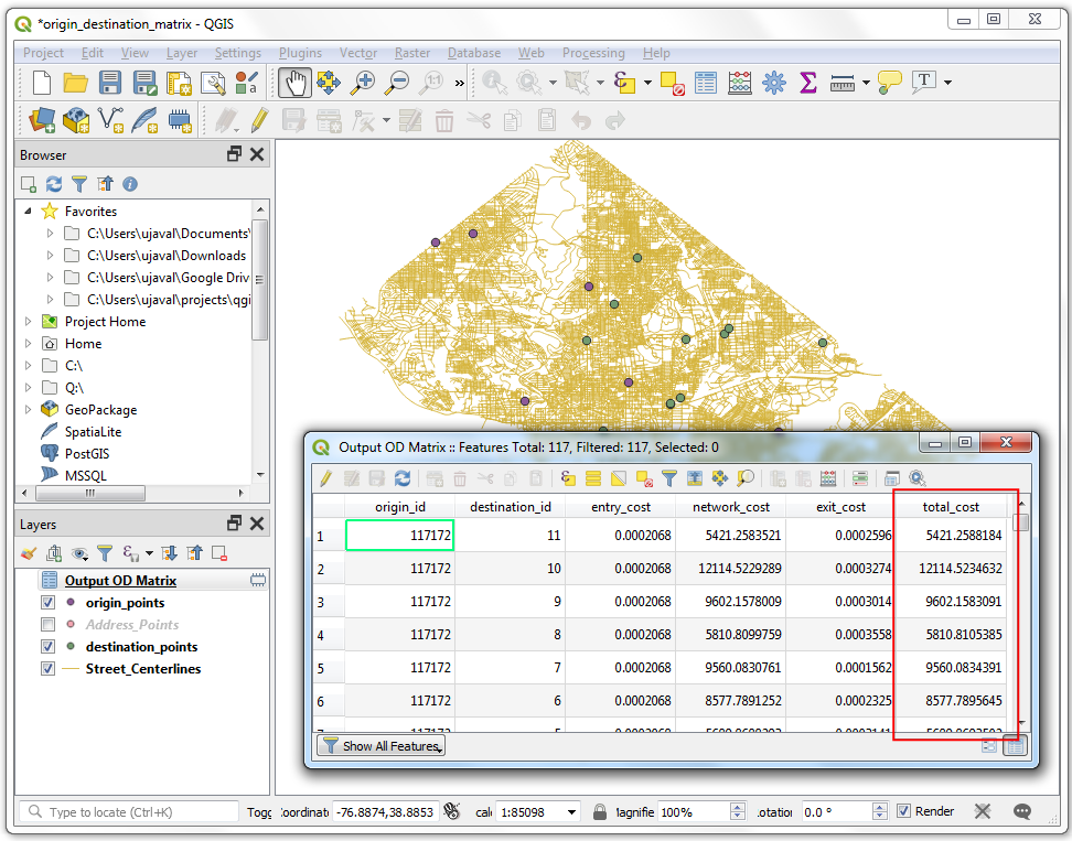
    origin_expr = QgsExpression('OBJECTID={}'.format(f['origin_id']))
    destination_expr = QgsExpression('OBJECTID={}'.format(f['destination_id']))
    origin_feature = origin_layer.getFeatures(QgsFeatureRequest(origin_expr))
    origin_coords =  [(f.geometry().asPoint().x(), f.geometry().asPoint().y())
        for f in origin_feature]
    destination_feature = destination_layer.getFeatures(QgsFeatureRequest(destination_expr))
    destination_coords =  [(f.geometry().asPoint().x(), f.geometry().asPoint().y())
        for f in destination_feature]
    params = {
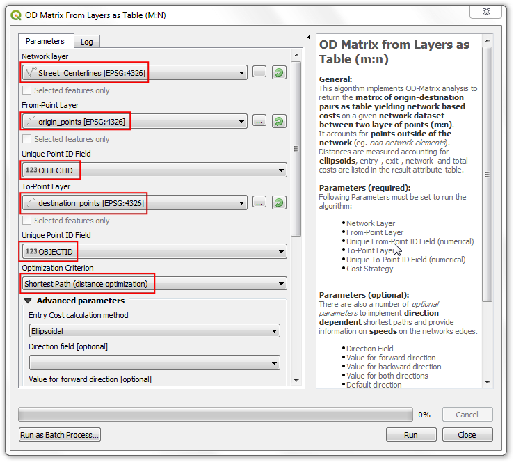
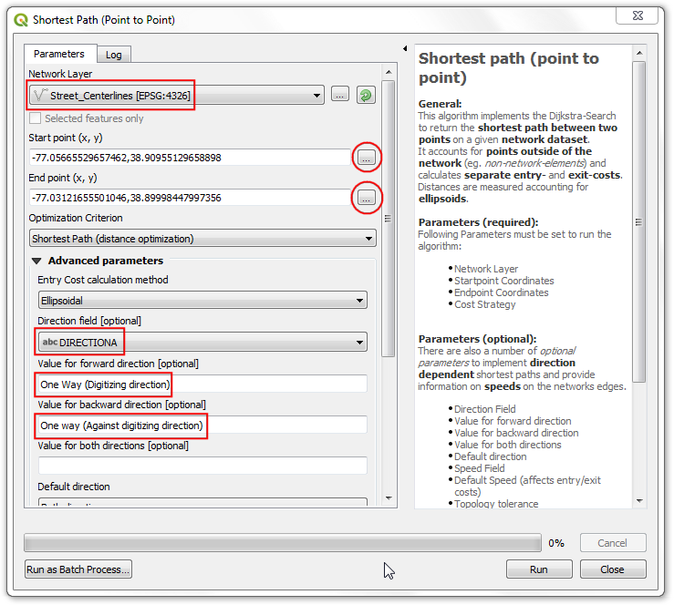
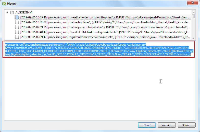
        'INPUT':'Street_Centerlines',
        'START_POINT':'{},{}'.format(origin_coords[0][0], origin_coords[0][1]),
        'END_POINT':'{},{}'.format(destination_coords[0][0], destination_coords[0][1]),
        'STRATEGY':0,
        'ENTRY_COST_CALCULATION_METHOD':0,
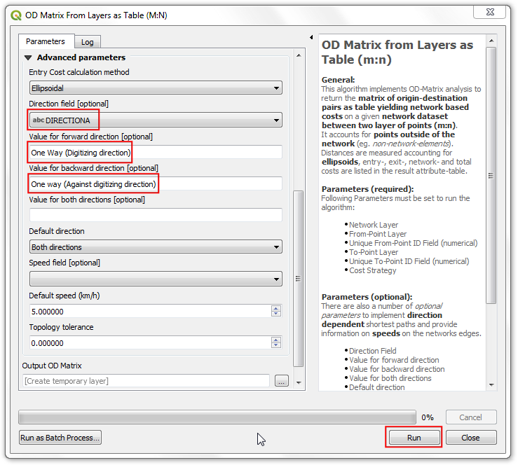
        'DIRECTION_FIELD':'DIRECTIONA',
        'VALUE_FORWARD':'One Way (Digitizing direction)\n',
        'VALUE_BACKWARD':'One way (Against digitizing direction)\n',
        'VALUE_BOTH':'',
        'DEFAULT_DIRECTION':2,
        'SPEED_FIELD':None,
        'DEFAULT_SPEED':5,
        'TOLERANCE':0,
        'OUTPUT':'memory:'}
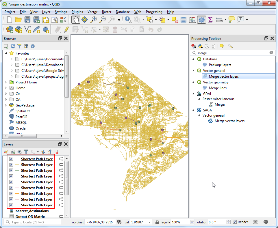
    print('Executing analysis')
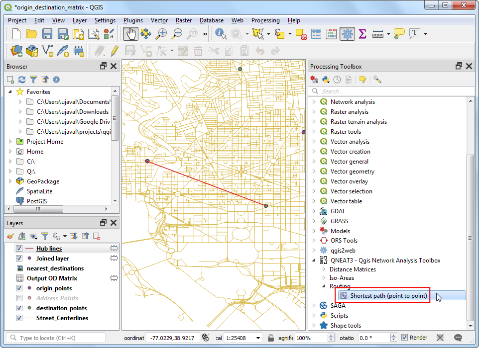
    processing.runAndLoadResults("qneat3:shortestpathpointtopoint", params)

The script will take a few minutes to run. Once finished, you will see 9 new layers named Shortest Path layer. Let’s merge these paths to a single layer. Find the Vector general ‣ Merge vector layers algorithm and launch it.

Select all 9 Shortest Path layer as the Input layers. Click Run.

A new Merged layer will be created which will contain shortest path between our origins and destinations.

Author

Subscribe to my mailing list

Change Language