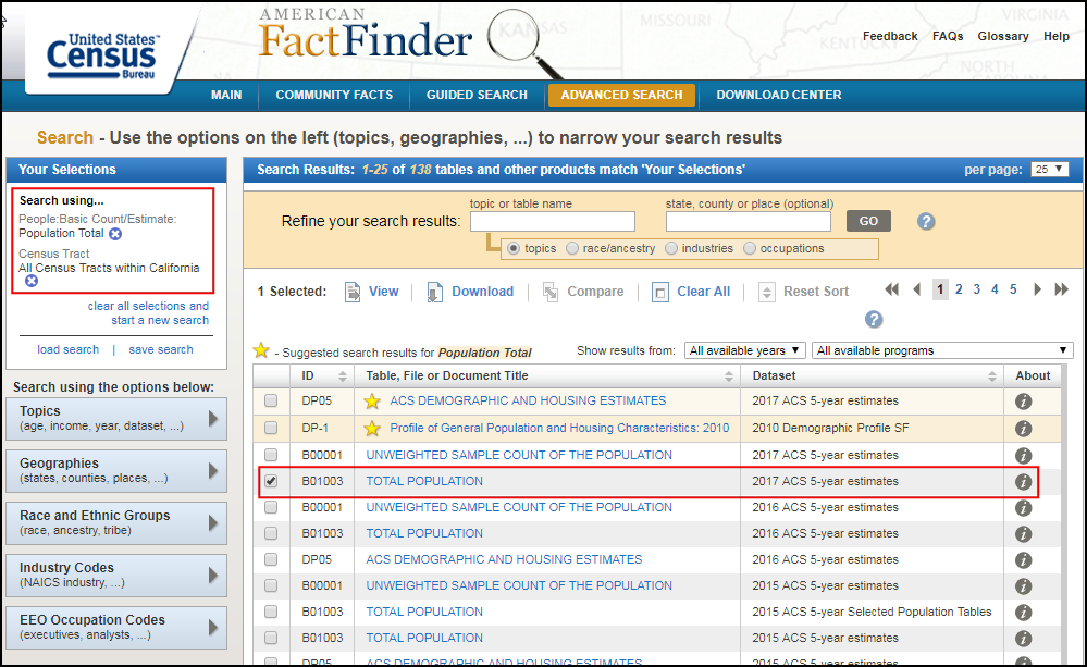
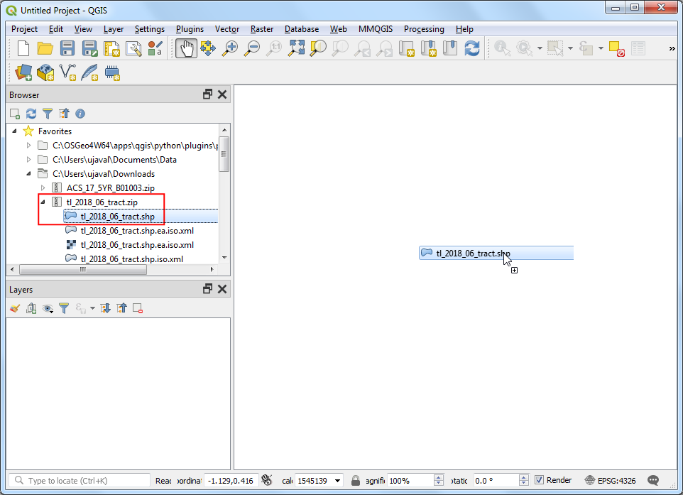
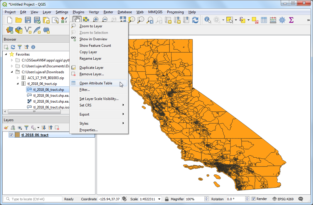
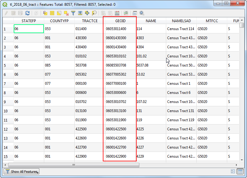
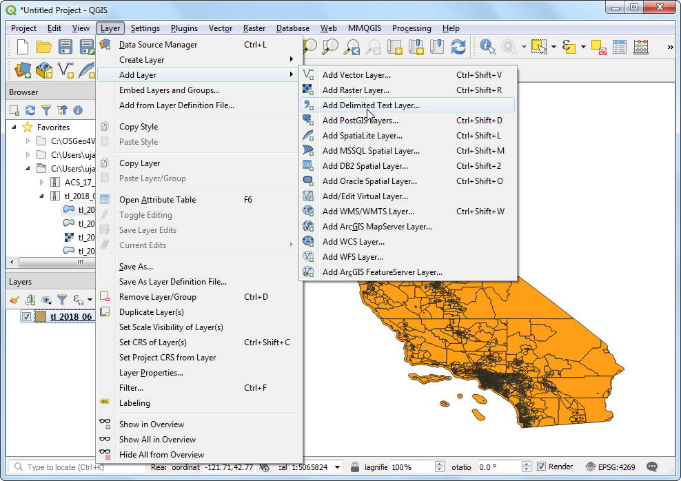
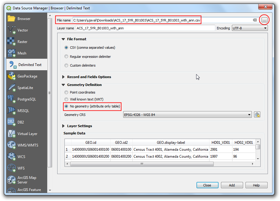
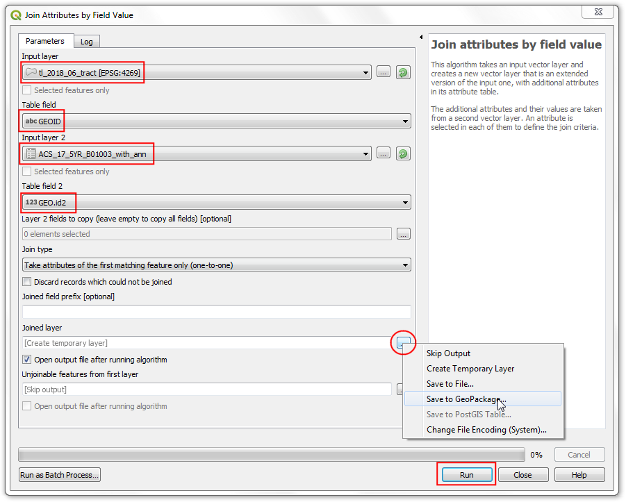
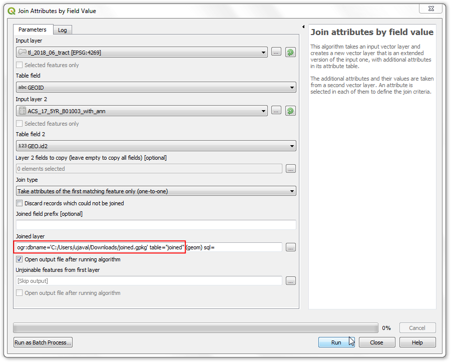
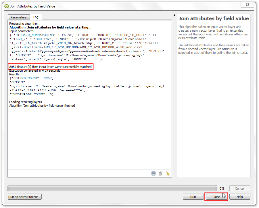
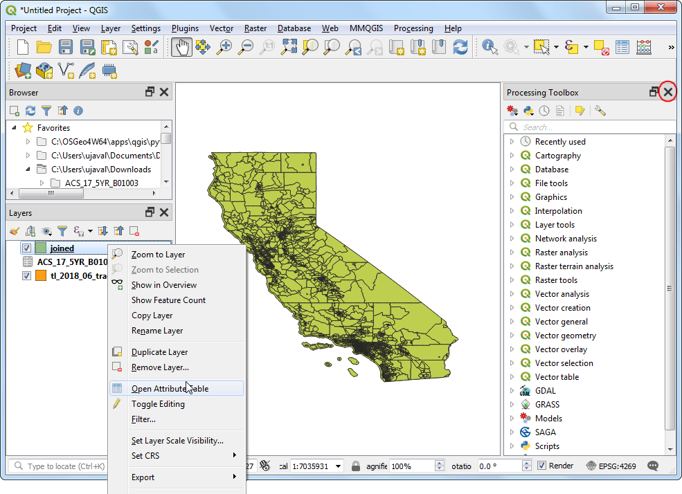
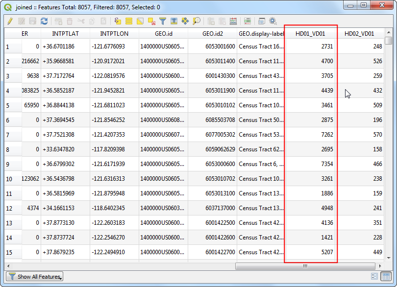
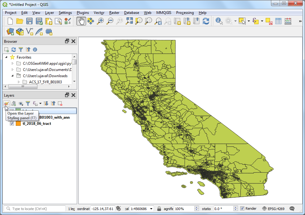
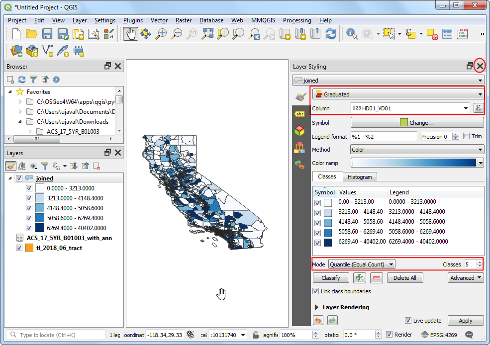
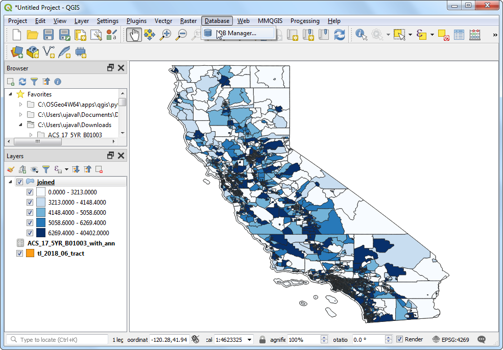
Performing Table Joins (QGIS3)¶

Overview of the task¶

We will use a shapefile of census tracts for California and population data table from US Census Bureau to create a population map for california.

Get the data¶

US Census Bureau provides TIGER/Line Shapefiles. You can visit the FTP site and download census tracts shapefile for California. Download Census Tracts for California file.

Americal FactFinder is a repository of all census data for the US. You can use Advanced Search and query for the Topic - Basic Count/Estimate and Geographies - All Census Tracts in California to create a custom CSV and download it. This tutorial uses TOTAL POPULATION | 2017 ACS 5-year estimates data.

For convenience, you may directly download a copy of both the datasets from the links below:

tl_2018_06_tract.zip

ACS_17_5YR_B01003.zip

Data Source [TIGER] [USCENSUS]

Procedure¶

1. Locate the tl_2018_06_tract.zip file in the QGIS Browser and expand it. Select the tl_2018_06_tract.shp file and drag it to the canvas.

2. You will see the layer tl_2018_06_tract loaded in the Layers panel. This layer contains the boundaries of census tracts in California. Right-click on the tl_2018_06_tract layer and select Open Attribute Table.

3. Examine the attributes of the layer. To join a table with this layer, we need a unique and common attribute for each feature. In this case, the GEOID field is a unique identifier for each tract and can be used to link this layer with any other layer or table containing the same ID.

4. Unzip the ACS_17_5YR_B01003.zip file and open the ACS_17_5YR_B01003_with_ann.csv file in a text editor. You will notice that each row of the file contains information about a tract along with the unique identifier we saw in the previous step. Note that this field is called GEO.id2 in the CSV. You will also note that the HD01_VD01 column has population value for each of the census tract.

5. Before importing this CSV file, we need to make a minor edit. QGIS CSV importer expects the first row of the file to contain the column headers and all remaining rows to contain the data for these columns. This file contains an extra row 2 with column labels. Delete that row and save the file.

6. Now we are ready to import the CSV file to QGIS. Go to Layer ‣ Add Layer ‣ Add Delimited Text Layer.

7. In the Data Source Manager window, click the ... button and browse to the CSV file and select it. Make sure you have selected File format as CSV (comma separated values). Since we are importing this as a table, we must specify that our file contains no geometry using the No geometry (attribute table only) option. Verify that Sample Data preview at the bottom looks fine and click Add followed by Close.

8. The CSV will now be imported as a table to QGIS and will appear as ACS_17_5YR_B01003_with_ann in the Layers panel. Now we are ready to create the table join. Go to Processing ‣ Toolbox.

9. First we need to change a default setting in the Processing Toolbox. Click the Options button.

10. In the Processing Options tab, check the Use filename as layer name option. When using algorithms from Processing Toolbox, this option makes the output layer names much more intuitive and useful. Click OK.

11. Back in the Processing Toolbox, search and locate the Vector General ‣ Join attributes by field value algorithm and double-click it to open it.

12. In the Join Attributes by Field Values dialog, select tl_2018_06_tract as Input layer and GEOID as the Table field. Select ACS_17_5YR_B01003_with_ann as the Input layer 2 and GEO.id2 as the Table field 2. Leave other options to their default values and click the ... button to select the output file location and select Save to GeoPackage....

13. Name the output geopackage as joined.gpkg and the output layer as joined. Click Run.

14. Once the processing finishes, verify that the algorithm was successful and click Close.

15. You will see a new layer joined loaded in the Layers panel. At this point, the fields from the CSV file are joined with the census tracts layer. You can close the Processing Toolbox for now. Right-click on the joined layer and select Open Attribute Table.

16. You will see a new set of fields, including the HD01_VD01 field containing population estimates.

17. Now that we have the population data in the census tracts layer, we can style it to create a visualization of population distribution. Select the joined layer and click the Open the Layer Styling Panel button.

18. In the Layer Styling panel, select Graduated from the drop-down menu. As we are looking to create a population map, we want to assign different color to each census tract feature based on the population estimate. Select HD01_VD01 as the Column. Select a color ramp of your liking from the Color ramp drop-down. In the Mode, select Quantile (Equal Count) with 5 Classes. Click the Classify button and see the map layer update with a color assigned to a population range. You can close the Layer Styling panel once you are satisfied with the map.

19. A good practice in any GIS analysis is to validate your results. To check our work, we can run some simple queries on the output layer to make sure the results are correct. Go to Database ‣ DB Manager....

20. All layers loaded in QGIS are available as Virtual Layers that can be queried using SQL without loading them into a separate database. This add a lot of useful functionality by enabling spatial and non-spatial SQL queries via SQLite engine and the Spatialite library. Locate the output layer from Virtual Layers ‣ Project layers ‣ joined` and select it. Click the SQL Window button.

21. Type the following query that sums the HD01_VD01 field to count the total population of the state. Enter the query in the Query tab and click Execute. The result will appear in the bottom panel. You can verify that the result matches the population of California.

select sum(HD01_VD01) as population from joined

22. SQL queries are also well-suited to perform group statistics. Here’s a query that sums the population field but adds a group by clause to group all census tracts by county and create a table of total population by county. The query also sorts the result by population. We can also cross-verify that the county with FIPS id 037 (Los Angeles County) is the most populated county in california .

select COUNTYFP as county, sum(HD01_VD01) as population
from joined group by COUNTYFP order by population desc