Running Processing Algorithms via Python (QGIS3)
The Processing Toolbox in QGIS contain an ever-growing collection of geoprocessing tools. The toolbox provides an easy batch processing interface to run any algorithm on a large number of inputs. See Batch Processing using Processing Framework (QGIS3). But there are cases where you need to incorporate a little bit of custom logic in your batch processing. As all the processing algorithms can be run programmatically via the Python API, you can run them via the Python Console. This tutorial shows how to run a processing algorithm via the Python Console to perform a custom geoprocessing task in just a few lines of code. Please review the Getting Started With Python Programming (QGIS3) tutorial to get familiar with the basics of the Python Scripting environment in QGIS.
Overview of the Task
We will use 12 gridded raster layers representing precipitation for each month of year and calculate average monthly rainfall for all zip codes in the Seattle area.
Other skills you will learn
- How to delete a column (i.e. field) from a vector layer.
Procedure
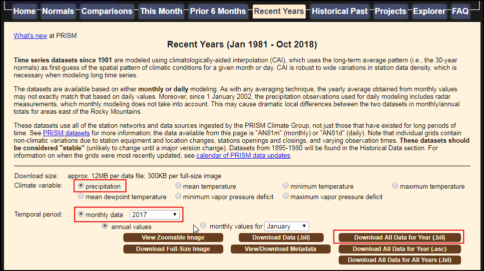
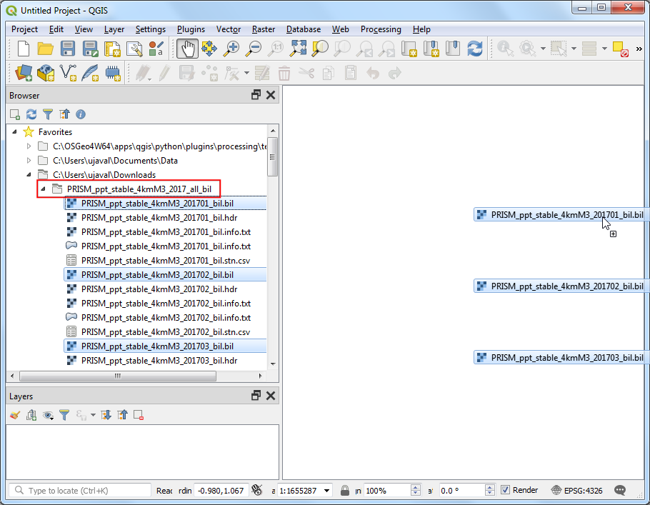
- Unzip the
PRISM_ppt_stable_4kmM3_2017_all_bil.zip file. Locate the PRISM_ppt_stable_4kmM3_2017_all_bil folder in the QGIS Browser and expand it. The folder contains 12 individual layers for each month. Hold the Ctrl key and select the .bil files for all 12 months. Once selected, drag them to the canvas.
Note
The data is provided in the BIL format. Each layer is presented with a set of files .bil file containing the actual data, a .hdr file describing the data structure and a .prj file containing the projection information. QGIS can load the .bil file and provided the other files exist in the same directory.
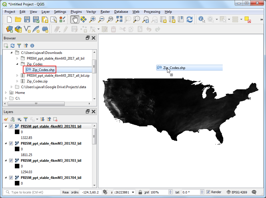
- Next, unzip the
Zip_Codes.zip file and extract the shapefile to a folder. Locate the Zip_Codes folder and expand it. Drag the Zip_Codes.shp file to the canvas.
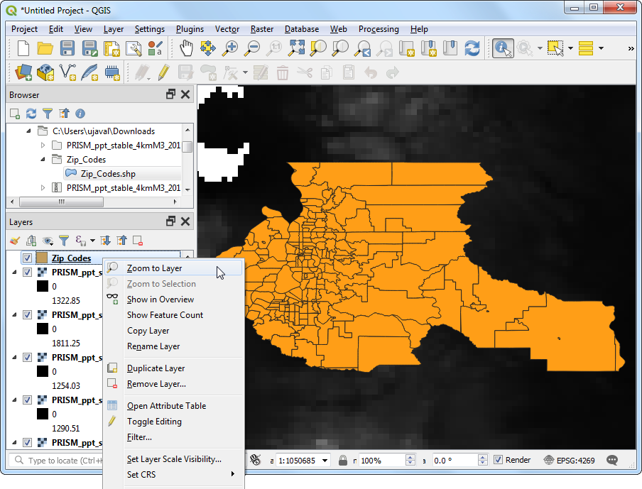
- Right-click the
Zip_Codes layer and select Zoom to Layer. You will see the zip code polygons for the city of seattle and neighboring areas.
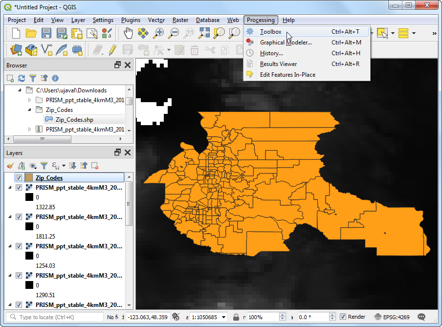
- Go to .
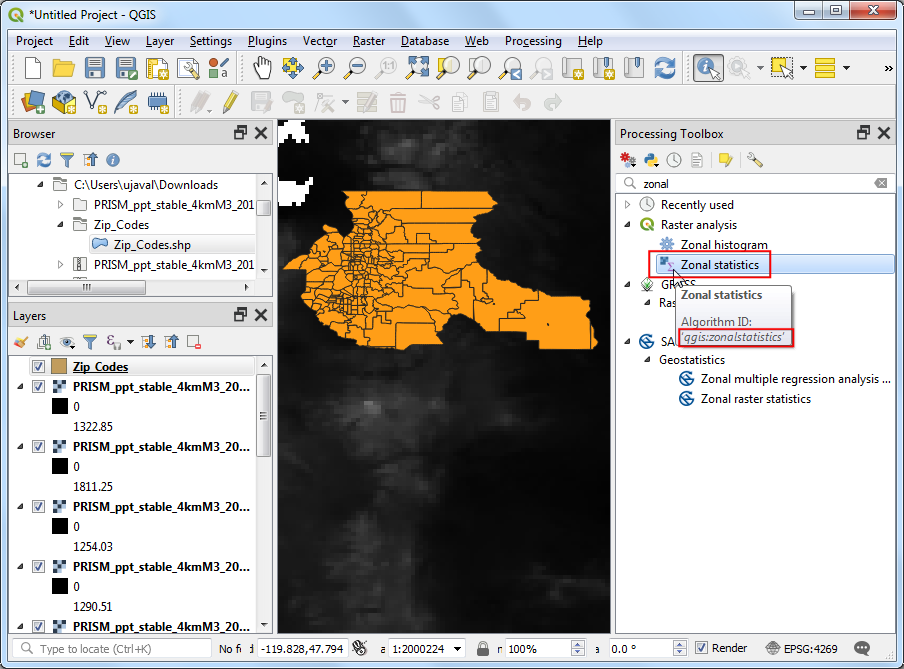
- The algorithm to sample a raster layer using vector polygons is known as
Zonal statistics. Search for the algorithm in the Processing Toolbox. Select the algorithm and hover your mouse over it. You will see a tooltip with the text Algorithm ID: ‘qgis:zonalstatistics’. Note this id which will be needed to call this algorithm via the Python API. Double-click the Zonal Statistics algorithm to launch it.
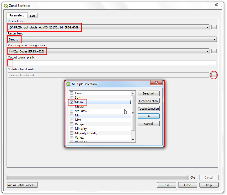
- We will do a manual test run of the algorithm for a single layer. This is a useful way to check if the algorithm behaves as expected and also an easy way to find out how to pass on relevant parameters to the algorithm when using it via Python. In the Zonal Statistics dialog, select
PRISM_ppt_stable_4kmM3_201701_bil as the Raster Layer and Zip_Codes as the Vector layer containing zones. Leave other paramters to default. Click the ... button next to Statistics to calculate and select only Mean. Click Run.
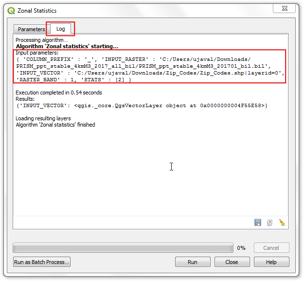
- Once the algorithm finishes, switch to the Log tab. Make a note of the Input Parameters that were passed to the algorithm. Click Close.
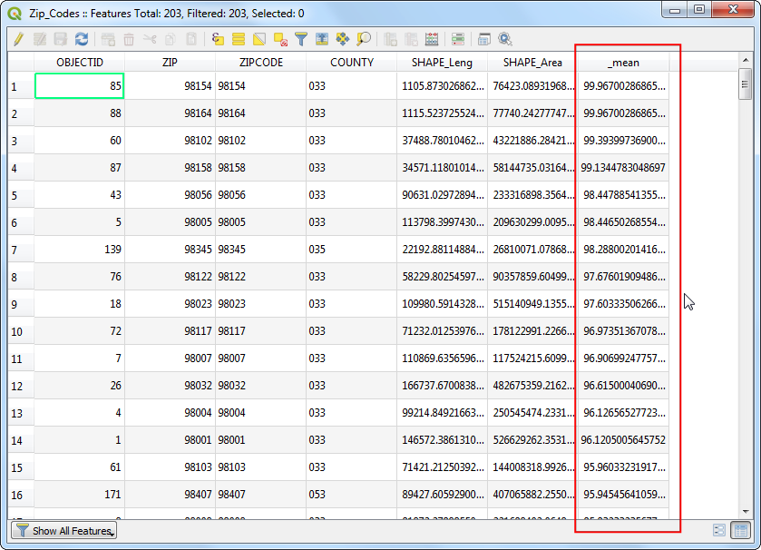
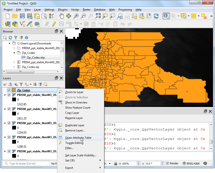
- Let’s check the results of the test run. In the main QGIS window, right-click the
Zip_Codes layer and select Open Attribute Table. This particular algorithm modifies the input zone layer in-place and adds a new column for every statistic that was selected. As we had selected only Mean value, a new column named _mean is added to the table. The _ was the default prefix. When we run the algorithm for layers of each month, it will be useful to specify a custom prefix with the month number so we can easily identify the mean values for each month (i.e. 01_mean, 02_mean etc.). Specifying this custom prefix is not possible in the Batch Processing interface of QGIS and if we ran this command using that interface, we would have to manually enter the custom prefix for each layer. If you are working with a large number of layers, this can be very cumbersome. Hence, we can add this custom logic using the Python API and run the algorithm in a for-loop for each layer.
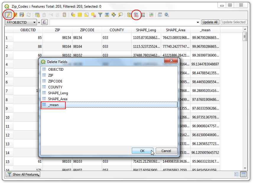
- Before we proceed, let’s delete the
_mean column that was created during our test run. Click the Toggle Editing mode button, followed by Delete field button. Select the _mean field and click OK.
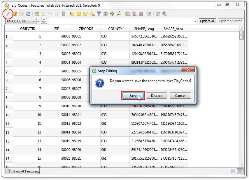
- Click the Toggle Editing mode button again and Save the changes.
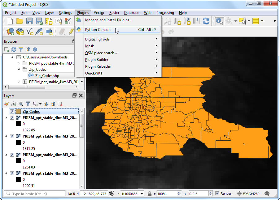
- Back in the main QGIS window, go to .
- To run the processing algorithm via Python, we need to access names of all the layers. Enter the following code in the Python Console and hit
Enter. You will see the names of all layers printed in the console.
root = QgsProject.instance().layerTreeRoot()
for layer in root.children():
  print(layer.name())
- For adding a custom prefix, we need to look at the layer name and extract a substring representing the month number. Enter the following code to iterate over all raster layers, extract the custom prefix and run the
qgis:zonalstatistics algorithm using it.
root = QgsProject.instance().layerTreeRoot()
for layer in root.children():
  if layer.name().startswith('PRISM'):
    prefix = layer.name()[-6:-4]
    params = {'INPUT_RASTER': layer.name(), 'RASTER_BAND': 1, 'INPUT_VECTOR': 'Zip_Codes', 'COLUMN_PREFIX': prefix+'_', 'STATS': 2}
    processing.run("qgis:zonalstatistics", params)
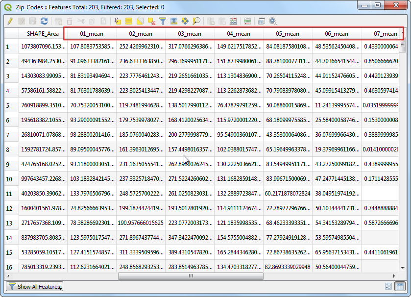
- Once the processing finishes, right-click on the
Zip_Codes layer and select Open Attribute Table.
- You will see 12 new columns added to the table with custom prefixes and mean precipitation values extracted from the raster layers.