Sampling Raster Data using Points or Polygons (QGIS3)
Many scientific and environmental datasets come as gridded rasters. Elevation data (DEM) is also distributed as raster files. In these raster files, the parameter that is being represented is encoded as the pixel values of the raster. Often, one needs to extract the pixel values at certain locations or aggregate them over some area. This functionality is available in QGIS via processing algorithms. Sample raster values for point layers and Zonal Statistics for polygon layers.
Overview of the task
Given a raster grid of daily maximum temperature in the continental US, we need to extract the temperature at a point layer of all urban areas and calculate the average temperature for a polygon layer of each county in the US.
Other skills you will learn
- Select and remove multiple layers from QGIS Table of Contents.
Procedure
- Unzip and extract both
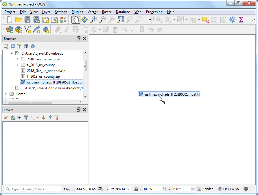
2018_Gaz_ua_national.zip and tl_2018_us_county.zip to a folder on your computer. Open QGIS and locate the us.tmax_nohads_ll_20190501_float.tif file in the QGIS Browser drag it to the canvas.
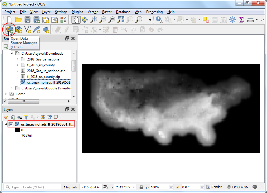
- You will see a new raster layer
us.tmax_nohads_ll_20190501_float loaded in the Layers panel. This raster layer contains the maximum temperature recorded at each pixel in degrees Celsius. Next we will load the urban areas point file. This file comes as a text file in the Tab Separated Values (TSV) format. Click the Open Data Source Manager button on the Data Source Toolbar.
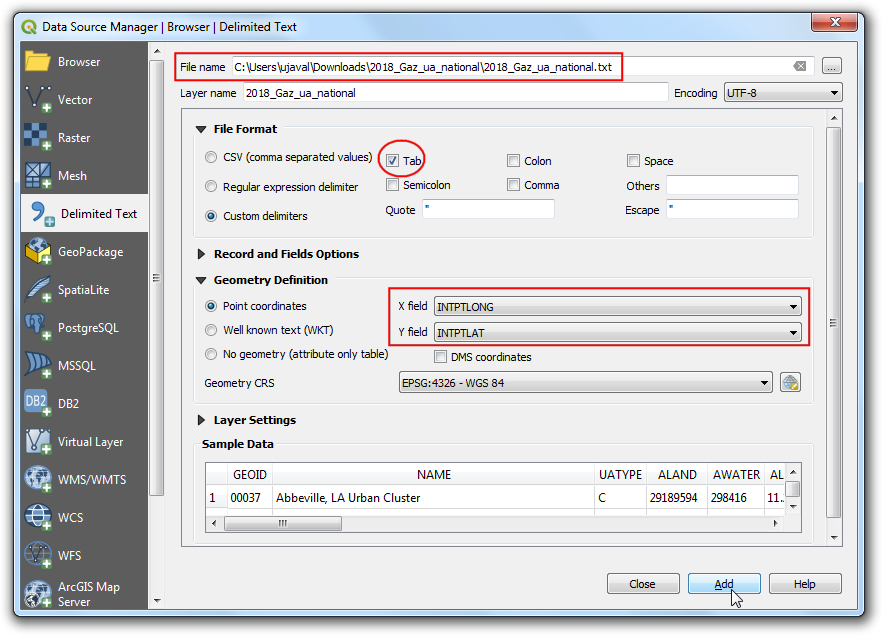
- Switch to the Delimited Text tab. Click the ... button next to File name and specify the path to the text file you downloaded. In the File format section, select Custom delimiters and check Tab. Select
INTPTLONG as the X field and INTPTLAT as the Y field. Click Add and then Close.
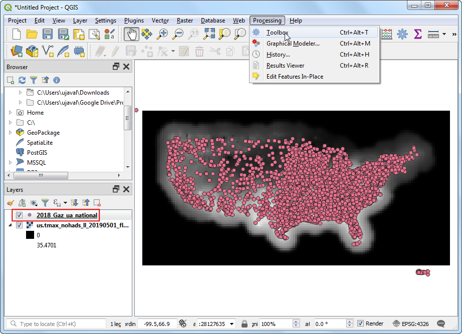
- A new point layer
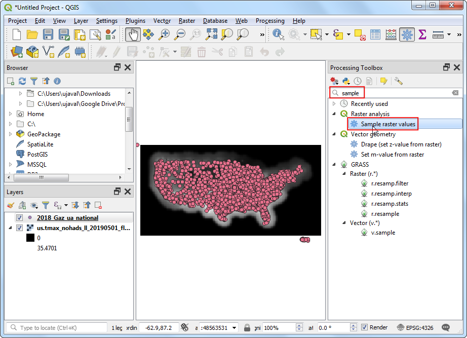
2018_Gaz_ua_national will be loaded in the Layers panel. Now we are ready to extract the values from the raster layer at these points. Go to .
- Search and locate the algorithm. Double-click to launch it.
- Select
2018_Gaz_ua_national as the Input Point Layer. Select us.tmax_nohads_ll_20190501_float as the Raster Layer to sample. Expand the Advanced parameters and enter tmax as the Output column prefix. Click Run. Once the processing finishes, click Close.
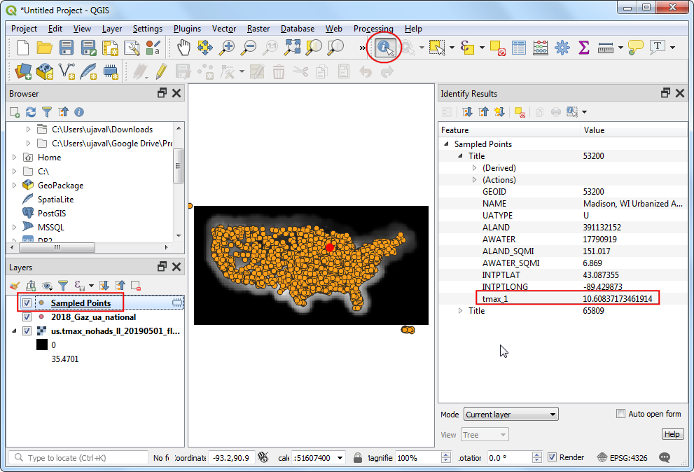
- A new layer
Sampled Points will be loaded in the Layers panel. Select the Identify tool in the Attributes Toolbar and click on any point. You will see the attributes displayed in the Identify Results panel. You will see a new attribute called tmax_1 added to each feature. This is the pixel value of the raster layer extracted at the point’s location. The 1 represents the band number of the raster. If the raster layer had multiple bands, you would see multiple new columns in the output layer.
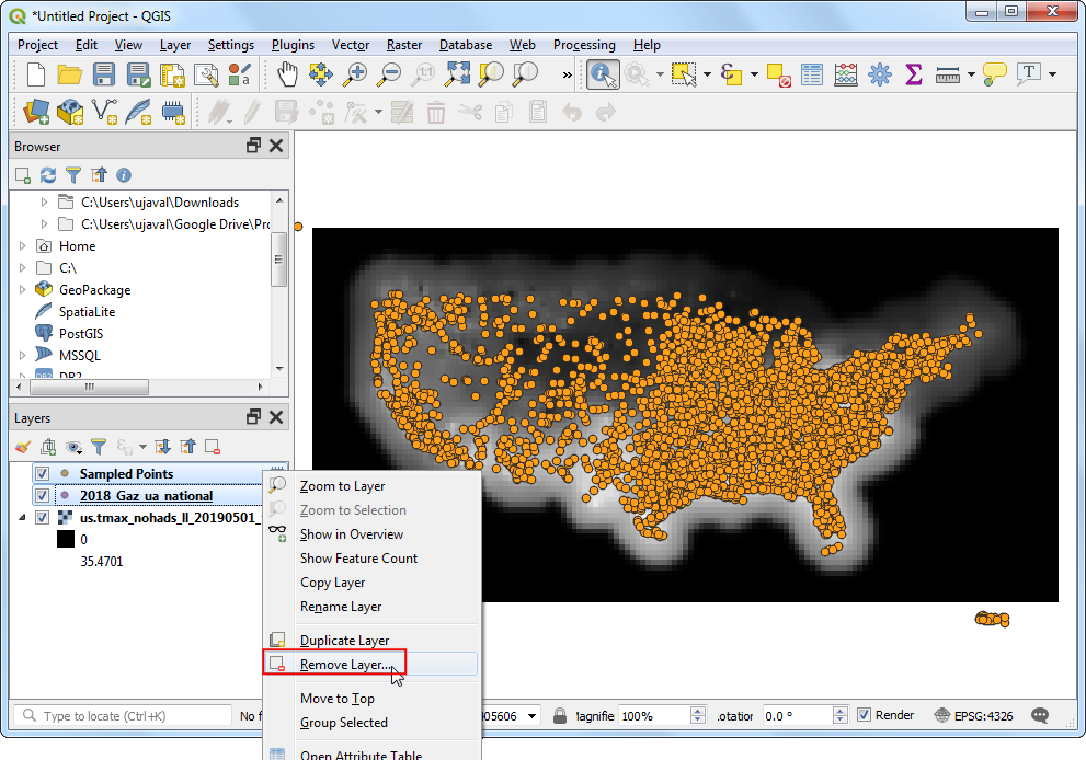
- First part of our analysis is over. Let’s remove the unnecessary layers. Hold the
Shift key and select Sampled Points and 2018_Gaz_ua_national layers. Right-click and select Remove to remove them from QGIS. When prompted for Remove 2 legend entries?, select OK.
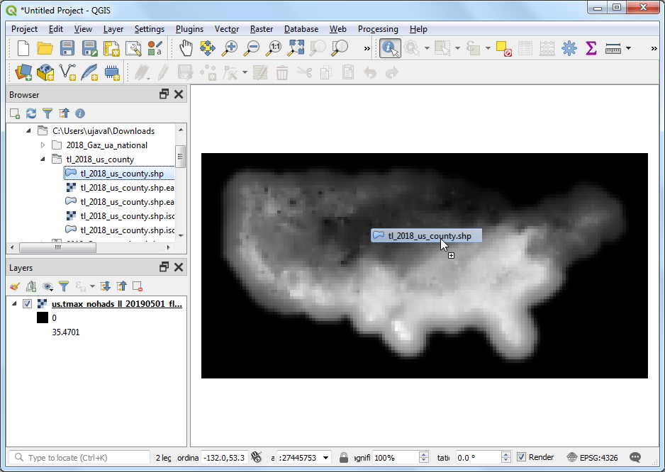
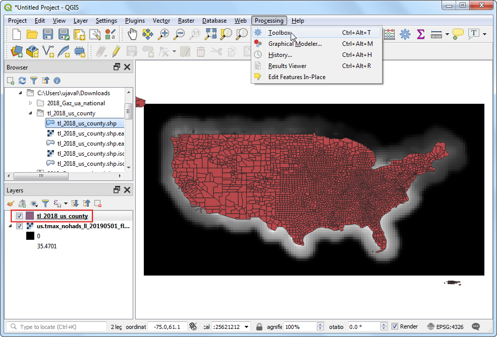
- Now we will use the counties layer to sample the raster and calculate average temperature for each county. Locate the
tl_2018_us_county.shp file in the QGIS Browser drag it to the canvas.
Note
Most processing algorithms will read the input layer and create a new layer. But the Zonal Statistics algorithm is different. It modifies the input layer and adds new attributes to it. That’s why it is important to unzip the input files first. QGIS can load a layer from a zip archive directly, but it cannot modify a zipped layer. The processing algorithm will fail if it cannot update the input layer.
- A new layer
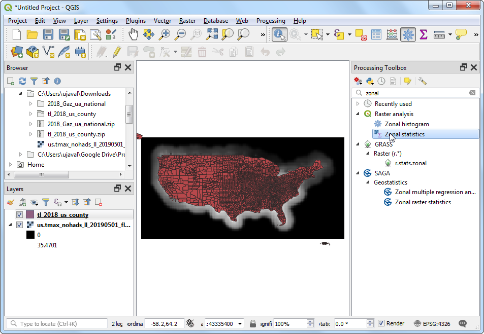
tl_2018_us_county will be loaded to the Layers panel. Go to .
- Search and locate the algorithm and double-click to launch it.
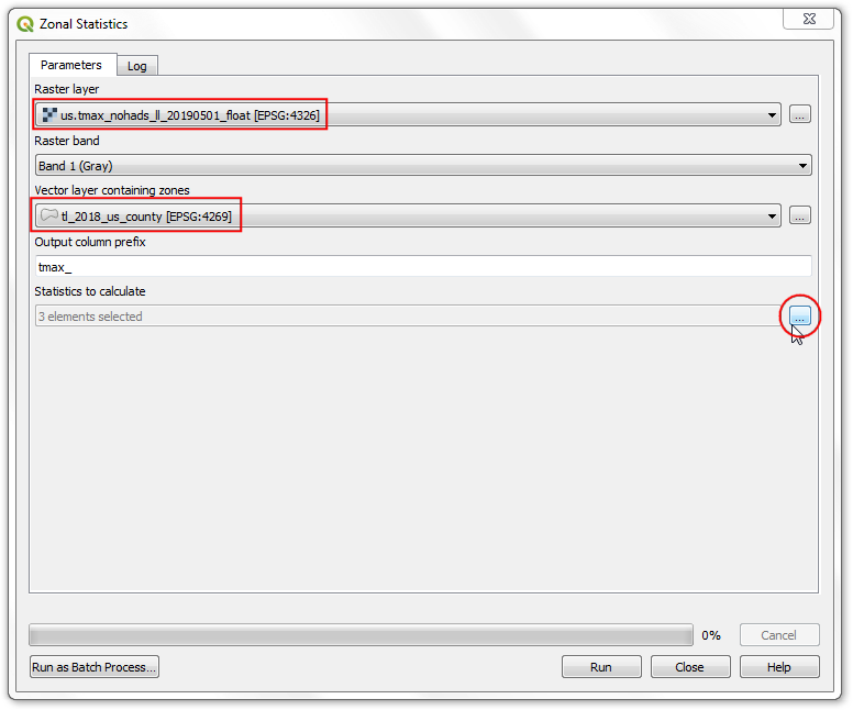
- Select
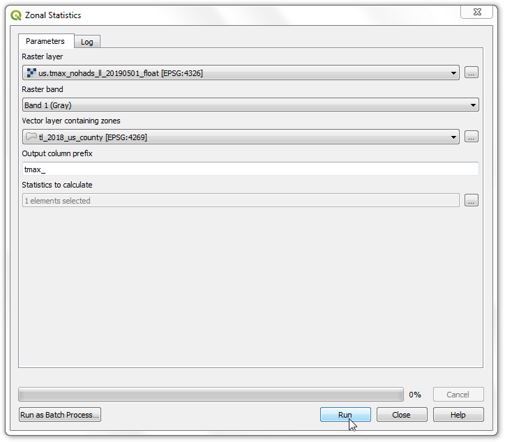
us.tmax_nohads_ll_20190501_float as the Raster layer and tl_2018_us_county as the Vector layer containing zones. Enter tmax_ as the Output column prefix. Click the ... next to Statistics to calculate.
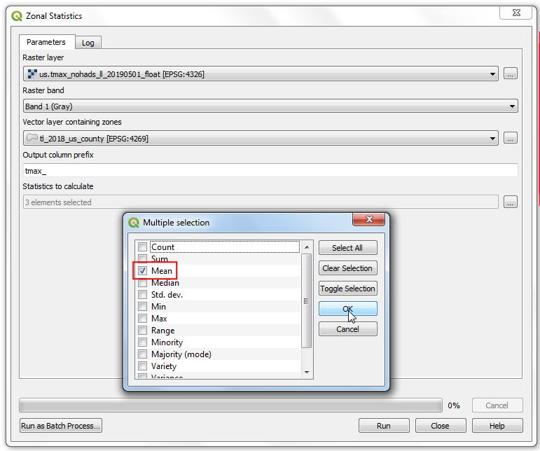
- Select only the
Mean value and click OK.
- Click Run to start the processing. The algorithm may take a few minutes to complete. Click Close.
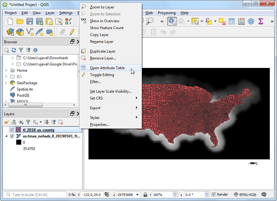
- As noted earlier, the Zonal Statistics algorithm doesn’t create a new layer, but modifies the zone layer. Right-click the
tl_2018_us_county layer, and select Open Attribute Table.
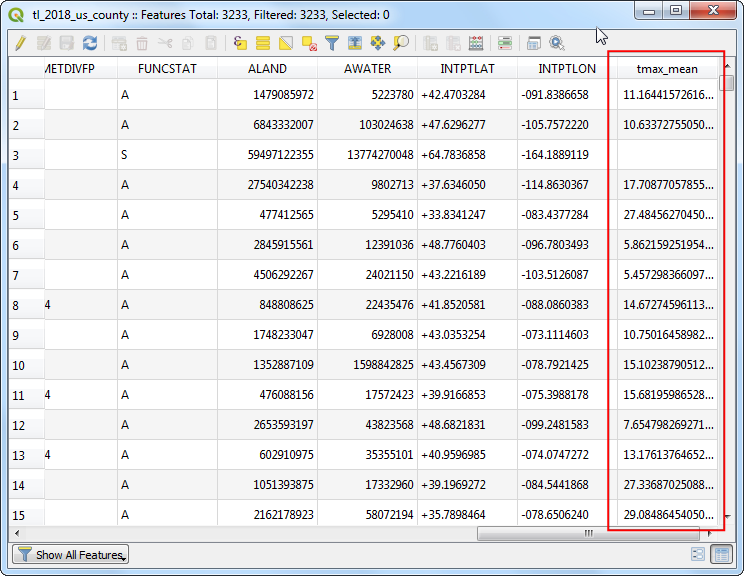
- You will see a new column called
tmax_mean added to the attribute table. This contains the average temperature value extracted over the polygon for each feature. There are some null values because those counties (belonging to Alaska, Hawaii and Puerto Rico) are outside of the raster layer’s extent.